Twenty-two identical, perfectly attentive simulated drivers on a 230 m ring road produced a stop-and-go jam out of nothing, and that jam rolled backward around the ring at 21.7 km/h while every car kept moving forward. Nobody braked, nobody crashed, and there was no obstacle. The only disturbance in the whole run was a single car nudged 0.5 m out of place at the start.
In 2008, Sugiyama and colleagues ran this experiment with real cars. They put 22 vehicles on a circular track, asked the drivers to cruise at about 30 km/h, and watched a jam form anyway. The paper became a classic because it removed every excuse: a circle has no merges, no exits and no bottleneck, so the jam could only come from the traffic itself. I asked K-Dense Web to rebuild that experiment in a computer with the Bando optimal velocity model, confirm that the jam emerges on its own, and measure how it moves.
The result was a 14-page illustrated report with 42 references, five figures and an animation of the ring. The part I want to highlight in this post, though, is not the report itself. It is how much of the session went into verification: the agent kept testing its own numbers against theory, against the original paper and against itself, and it reported the places where the model does not match reality. You can browse the full session, including every script and result file, here.
The Jam Builds Itself
The model gives every driver the same rule: look at the gap to the car ahead, decide what speed feels right for that gap, and accelerate or brake toward it with a short delay. There is no noise, no aggressive driver and no random event. The agent calibrated the model so that perfectly uniform traffic on this ring would move at exactly 30 km/h, the speed the real drivers were asked to hold.
Before choosing parameters, it wrote down seven acceptance criteria (the uniform flow must be unstable, no car may overtake another, cars must stay at least one 4.4 m car length apart, and so on) and a rule for picking among the survivors. It then screened 96 parameter combinations against those criteria. Eleven passed, and the pre-declared rule selected one of them. Deciding the criteria before looking at the results matters, because it prevents the quiet tuning that makes a simulation look better than it is.
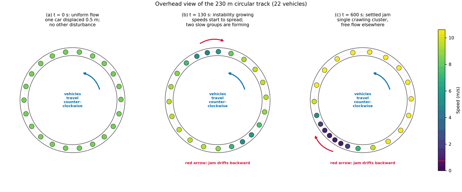 Overhead view of the 22 simulated cars, colored by speed. (a) At the start, the cars are evenly spaced, and one car has been displaced by 0.5 m. (b) At 130 s, speeds have started to spread and two slow groups are forming. (c) At 600 s, long after those groups have merged, a single cluster of slow cars (dark) occupies one arc of the ring while the rest of the ring runs freely (yellow). The red arrows show the jam drifting backward, against the traffic.
For the first minute and a half the ring looks calm. Then the small ripple grows: each driver's correction forces a slightly larger correction from the driver behind. By 90.6 s the spread in speeds has grown tenfold. Two slow clusters form first and then merge, and by about 270 s the system has settled into a single, permanent jam. The animation below shows the settled state, with one tracer car circled in red so you can follow it into and out of the jam.
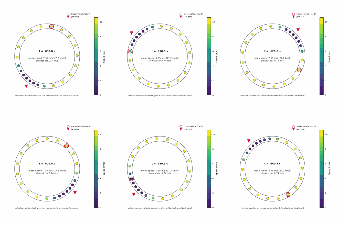 The circular track in the settled state. Cars drive counterclockwise, and the red triangle marks the jam core, which drifts clockwise. Watch the circled car slow down as it enters the cluster and speed up as it leaves.
The Jam Moves Backward
The space-time diagram is the clearest way to see what is happening. Each thin line is one car's path, and all of them slope upward, because every car always moves forward. The dark bands are where the cars are slow, and they slope the other way. The jam is a pattern of which cars are currently stuck, not a group of cars, so it can travel against the traffic.
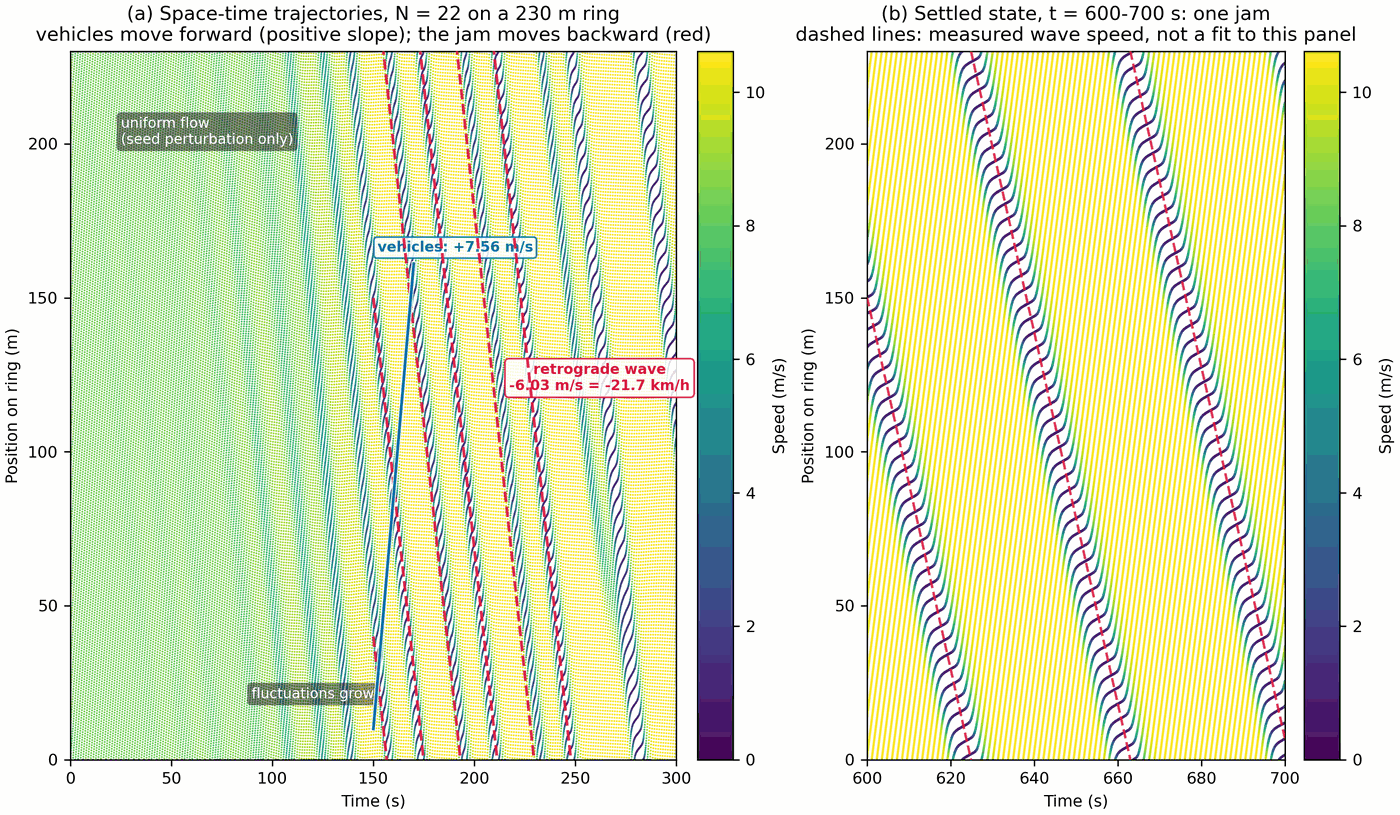 Left: the first five minutes. Smooth flow on the left breaks into dark jam bands on the right, and at this stage the ring still holds two jams. Right: 600 to 700 s, after the two jams have merged into one. The red dashed lines are drawn at the jam speed measured by a separate analysis and anchored at the slowest car at 600 s. They are an overlay of that independent value, not a line fitted to this picture.
The agent measured the jam speed three different ways. Tracking the slowest car and finding the tilt that best aligns the whole space-time pattern gave -6.0322 and -6.0323 m/s, which differ by only 0.00005 m/s (0.0009%). A third method, based on the time lag between neighboring cars braking, came out 1.3% faster. Instead of averaging it in, the agent explained why this method is biased by construction and reported it as a cross-check only. The headline is -21.72 km/h. The original paper reports "roughly 20 km/h" backward.
Verification Step 1: Predict First, Then Measure
The most convincing check in the session happened before the simulation was run. A standard linear stability calculation says whether smooth traffic will survive a small disturbance, and if not, how fast the disturbance should grow. For the chosen parameters it predicted that uniform flow is unstable, that the fastest-growing pattern has two clusters, and that it should grow with a characteristic time of 31.6 s.
The simulation then measured a growth time of 32.0 s (a fit over 903 data points, R² = 0.9996), and the dominant pattern during early growth was the predicted two-cluster mode. The measured and predicted growth rates agree to within 1.2%. That is a real test, because the prediction came from the equations alone and could have failed.
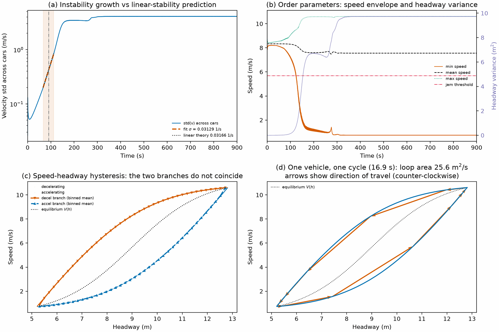 (a) The spread of speeds across the 22 cars over time, on a log scale. The orange dashed fit to the growth phase and the black dotted line from linear theory lie almost on top of each other. (b) The slowest, average and fastest speeds, with the variance of the gaps between cars. The later step near 280 s is the jam settling into a single cluster. (c, d) At the same gap, cars entering the jam move faster than cars leaving it, so each car traces a loop instead of a single curve.
The agent added a second, independent test after the session's methodology review. It reran the simulation from nine different starting disturbances, from a 0.05 m nudge to a 2 m nudge plus random disturbances on every car. The final jam speed varied by only 0.00002 m/s across all nine runs, and every run ended with exactly one cluster. Only the onset time changed, and it changed exactly as theory predicts: plotting onset time against the logarithm of the nudge size gave a slope of -30.9 s, against a predicted -31.6 s.
Verification Step 2: The Benchmarks Were Retrieved, Not Recalled
A common failure in AI-written science is comparing a result with a number the model remembers from a paper. Here the agent fetched the open-access Sugiyama paper during the session, converted it to text with the markitdown skill, and quoted every benchmark verbatim. The analysis script then checked programmatically that each quote actually appears in the converted text. All eight quotes were found.
Reading the source closely also changed the comparison. The paper reports every observable with words like "roughly" and "about", with no error bars, no video sampling rate and no tracking precision. The agent concluded that the source cannot support a precise statistical comparison, and said so, instead of inventing an uncertainty for the experiment.
| Observable | Experiment (quoted) | Simulation | Verdict |
|---|---|---|---|
| Jam speed | "roughly 20 km/h" backward | 21.72 km/h backward | Same direction and size |
| Speed outside the jam | "∼40 km/h" | 38.2 km/h | Close |
| Speed inside the jam | "stop completely" | 2.65 km/h | Model crawls, does not stop |
| Cars in the jam | "five vehicles" | 6.8 | Depends on the definition |
| Number of clusters | one | one | Match |
Verification Step 3: Report the Mismatches
The table above has two rows that do not match, and the agent treated both carefully instead of smoothing them over.
The first is the standstill. Real drivers in the experiment stopped completely, but the slowest simulated car crawls at 0.74 m/s. The agent traced this to the structure of the model: in the standard optimal velocity model a car only reaches zero speed when its gap shrinks to nearly zero, which would mean cars overlapping. To confirm the diagnosis, it added a minimum standstill gap to the model and reran it. With a gap of 5 m, a little over one car length, the jam core stops at 0.0005 m/s, and the backward wave survives almost unchanged (23.0 km/h instead of 21.7 km/h).
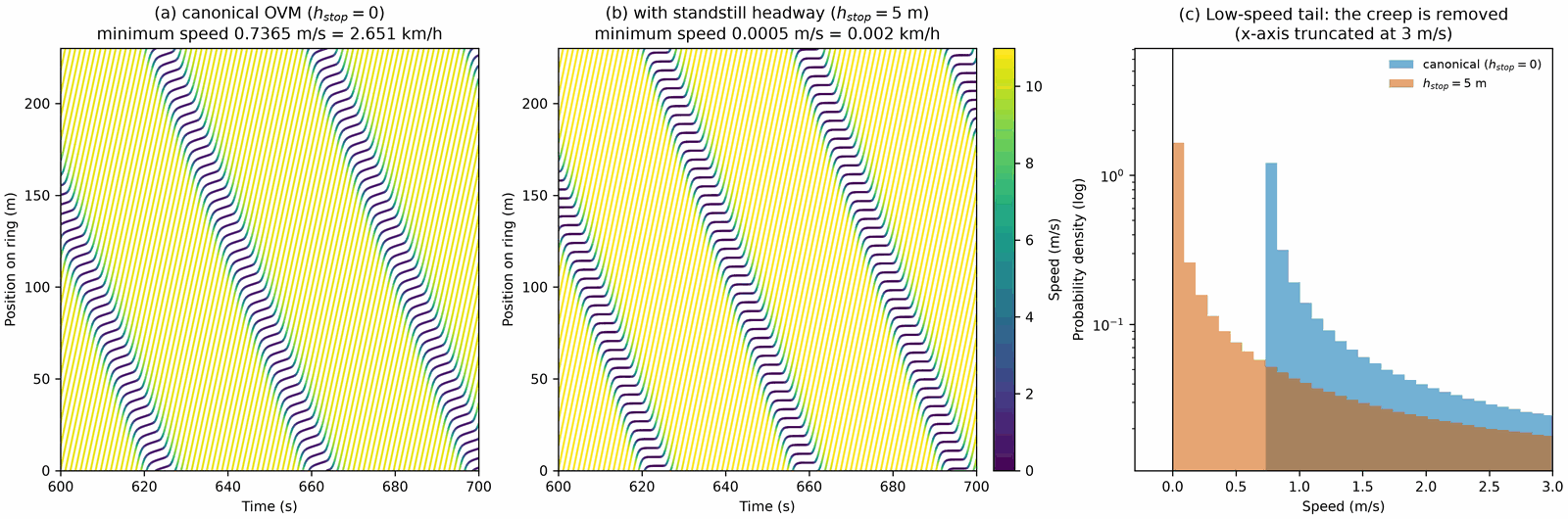 (a) The standard model: the slowest car still moves at 0.74 m/s. (b) With a 5 m standstill gap, the jam core comes to a genuine stop. (c) The low-speed distribution of both versions. The standard model cuts off sharply at 0.74 m/s, while the modified model extends to zero.
The second is the size of the jam. The simulation puts 6.8 cars in the jam, against the paper's five, but "in the jam" depends on how slow a car must be to count. Sweeping that threshold from 1 to 8 m/s moves the answer from 3.4 to 7.7 cars, and a 2 m/s threshold gives five. The agent pointed out that it found this threshold after it already knew the target, so it cannot count as agreement. Its conclusion was narrower: the quantity is not defined precisely enough on either side to support a comparison at all.
It flagged one more point that a reader could easily miss. The driver reaction time in the chosen model is about 0.42 s, which is quick for a human. Slower reactions were tested, and every one of them that formed a jam pushed cars closer than one car length, which would mean their bodies overlap. The report therefore states that the reaction time was forced by the no-overlap constraint and should not be read as a claim about real drivers.
The Agent Also Caught Its Own Errors
Several corrections in the session came from the agent checking its own work, and the README records each one. An early version computed gaps between cars in a way that let cars collide, pass through each other and reappear with a normal-looking gap, so the run looked healthy while being physically meaningless. The agent switched to a convention where the gaps must sum to the ring length (checked to 3 × 10⁻¹⁴ m) and a collision shows up as a negative gap.
The originally planned 300 s run turned out not to be stationary, because the pattern was still merging from two clusters into one, so the production run was extended to 900 s. One of the planned wave-speed methods was dropped after a sensitivity sweep showed it could be off by a factor of about 3.4 when the ring holds two unequal clusters. Even the figures were checked: the middle snapshot uses 130 s instead of the suggested 30 to 60 s, because the instability only becomes visible at 90.6 s, and an earlier panel would have looked identical to the starting state.
What the Deliverable Looks Like
The final output was written for a general audience: a 14-page PDF titled A Traffic Jam With No Cause, with boxes that explain how to read a space-time diagram and why a jam can move backward. It also includes the simulation code, every result file, a claim ledger that links each number to the file it came from, and the animation. Of the 42 references, 41 were resolved through the Crossref API and checked field by field against the returned record. The one reference without a DOI, a 1974 symposium paper, was checked against its record in the TRB transportation research database.
Why This Matters Beyond Traffic
The traffic result is fun, and it also carries a practical message. In this simulation every driver was flawless and identical, and the jam formed anyway. Compared with the smooth flow it started from, the jammed ring carried 9.3% less traffic with the same cars on the same road, because the average speed fell from 30 km/h to 27.2 km/h. (The report quotes 18.9%, which comes from averaging each car's own speed-to-gap ratio; counting the cars that pass a fixed point gives 9.3%.) This is the same mechanism behind field experiments in which a single smoothly driven autonomous vehicle damped stop-and-go waves on a ring of human drivers.
For me, the broader lesson is about how to trust a simulation. A model that produces a nice picture is easy to build. It is harder to show that the growth rate matches theory, that the result does not depend on the starting condition, that the benchmark values come from the source, and that the remaining mismatches are understood. That is the work this session did without being asked for each step.
Try it yourself at app.k-dense.ai, or browse the full session here.
Questions? Contact us at contact@k-dense.ai.